Contextual Bandit Theory: Regret Bounds and Exploration
Part 2 of 5: Theory That Informs Practice
TL;DR: Contextual bandits minimize regret—cumulative opportunity cost versus the optimal policy. Optimal algorithms achieve O(√(dT log T)) regret for d-dimensional contexts. The exploration-exploitation tradeoff is fundamental: confidence bounds (UCB) and posterior sampling (Thompson) provide principled solutions. This math directly guides algorithm selection and hyperparameter tuning.
Reading time: ~18 minutes
Introduction: Why Math Matters for Practice
You don’t need to derive regret bounds to deploy bandits in production. But understanding the mathematics directly informs practical decisions:
- Algorithm selection: Why LinUCB for linear rewards? Why Thompson Sampling often wins empirically?
- Hyperparameter tuning: What does α control in LinUCB? How to set it?
- Debugging: Why is my bandit not converging? (Check if regret is sublinear)
- Feature engineering: Why does dimensionality hurt? (√d penalty in regret bounds)
This post builds intuition for the theory that makes contextual bandits work.
The Contextual Bandit Problem (Formal)
Setup
At each round t = 1, 2, …, T:
- Environment reveals context xₜ ∈ X (context space)
- Agent chooses action aₜ ∈ A from available action set
- Environment generates reward rₜ ~ P(r | xₜ, aₜ) from unknown distribution
- Agent observes reward rₜ for chosen action (but not rewards for unchosen actions)
Goal
Learn policy π: X → A that maximizes expected cumulative reward:
Key Insight: Partial Feedback
We only observe rewards for actions we take. This is the partial feedback problem—we never know what would have happened if we’d chosen differently (the counterfactual outcome).
Example:
Context: User is 25-year-old in San Francisco
Action chosen: Recommend Product A
Reward observed: Click (reward = 1)

Unknown counterfactuals:
- What if we'd shown Product B? Maybe reward = 0 (worse)
- What if we'd shown Product C? Maybe reward = 1 (equally good)

We'll never know unless we try those actions in similar contexts.
This partial observability is why exploration is necessary—we must try actions to learn their value.
Regret: The Fundamental Performance Metric
Since we don’t know the true reward distributions, we can’t compute V(π) directly. Instead, we measure regret—how much worse we do compared to the optimal policy.
Definition
Let π* be the optimal policy that always chooses the best action for each context. The regret after T rounds is:
where rₜ* is the reward we would have gotten from the optimal action at time t.
Interpretation
Regret measures cumulative opportunity cost. If R(T) = 100 after 1000 rounds, we earned 100 less total reward than optimal.
Important: We want algorithms that minimize regret growth.
Sublinear Regret
An algorithm is good if regret grows sublinearly in T:
Equivalently, average regret goes to zero:
This means we’re converging to optimal performance. Linear regret R(T) = Θ(T) would mean we’re making a constant mistake forever—we never learn.
Typical Regret Bounds
| Algorithm | Regret Bound | Interpretation |
|---|---|---|
| ε-greedy | O(T^(2/3)) | Suboptimal. Explores forever at fixed rate. |
| UCB | O(√(T log T)) | Near-optimal for MAB. Confidence-based exploration. |
| Thompson Sampling | O(√T) | Optimal for many problems. Posterior sampling. |
| LinUCB | O(d√(T log T)) | Linear contextual bandit. Pays √d factor for d dimensions. |
The √T bound is essentially optimal—you can’t do better in the worst case. This comes from a fundamental information-theoretic tradeoff.
Visual Comparison of Regret Growth
Practical interpretation:
After 10,000 rounds:
- Linear O(T): ~10,000 cumulative regret (never learned)
- ε-greedy O(T^(2/3)): ~464 cumulative regret
- UCB O(√T log T): ~130 cumulative regret
- Thompson O(√T): ~100 cumulative regret
The difference compounds over time. In production with millions of decisions, UCB/Thompson save significant value vs ε-greedy.
Reward Models: Assumptions About Structure
Real-world reward functions are complex. We make modeling assumptions to make learning tractable.
Linear Reward Model
Assumption: Reward is a linear function of context features:
where:
- θₐ ∈ ℝᵈ is a weight vector for action a
- x ∈ ℝᵈ is the context vector
- ε ~ N(0, σ²) is noise
When this is reasonable:
✅ Features are well-engineered (embeddings, hand-crafted)
✅ Relationships are approximately linear in feature space
✅ Interpretability is important (coefficients show feature importance)
Limitations:
❌ Misses complex nonlinear interactions
❌ Requires good feature engineering upfront
❌ Can underfit when true function is highly nonlinear
Example: Content Recommendation
Context x: [user_age, user_tenure, content_freshness,
            content_popularity, topic_match]
Action a: show_content (binary)

Linear model:
r(x, show) = θ₁·age + θ₂·tenure + θ₃·freshness +
             θ₄·popularity + θ₅·topic_match

Interpretation: If θ₃ = 0.8, each unit increase in freshness
                adds 0.8 to expected reward
Generalized Linear Models (GLMs)
Assumption: Reward follows an exponential family distribution with linear predictor:
where g is a link function.
Common cases:
Logistic regression (binary rewards):
Use when reward is click/no-click, conversion/no-conversion.
Poisson regression (count rewards):
Use when reward is number of purchases, page views, etc.
Advantage: Captures bounded or discrete reward structures while maintaining interpretability.
Nonlinear Models (Neural Bandits)
Assumption: Reward is a complex nonlinear function:
where f is a neural network with parameters θₐ.
When this is necessary:
✅ Complex feature interactions that linear models can’t capture
✅ High-dimensional raw inputs (images, text)
✅ Sufficient data to train deep models
Challenges:
❌ Requires much more data
❌ Less interpretable (black box)
❌ Harder to quantify uncertainty (needed for exploration)
❌ Computationally expensive
When to use each:
| Context Dim | Reward Structure | Recommended Model |
|---|---|---|
| d < 50 | Linear or mildly nonlinear | Linear |
| d = 50-500 | Linear with interactions | Linear + feature engineering |
| d > 500 | Linear | Linear with regularization (large λ) |
| Any d | Highly nonlinear | Neural network |
| Images, text | Complex patterns | Neural (CNN, Transformer) |
The Exploration-Exploitation Tradeoff
This is the fundamental dilemma in bandit problems.
The Tension
Exploitation: Choose the action that has performed best so far. Maximize immediate reward based on current knowledge.
Exploration: Try actions with uncertain rewards. Gather information that might lead to better decisions later.
The conflict: Exploration sacrifices short-term reward for long-term learning. Exploitation maximizes current reward but risks missing better alternatives.
Toy Example
Two actions: A and B
Current estimates:
  μ̂_A = 0.8 (based on 100 trials)
  μ̂_B = 0.6 (based on 10 trials)

Pure exploitation: Always choose A (highest estimate)
Problem: B's estimate is uncertain. True μ_B might be 0.9,
         but we have sparse data.

Pure exploration: Choose randomly to gather data
Problem: While gathering data, we're not maximizing reward

Optimal balance: Choose A most of the time, occasionally try B
                 until confident about its value
Mathematical Formalization
Define the exploitation gap as the difference between estimated best and true best:
And the exploration benefit as information gain:
Optimal policies balance these:
where λ controls exploration intensity.
Visual Representation
Why This Matters in Practice
If you over-exploit (ε = 0.01):
- Converge quickly to locally optimal solution
- Miss potentially better alternatives
- Regret grows linearly if you lock onto suboptimal action
If you over-explore (ε = 0.5):
- Waste traffic on clearly inferior actions
- Slow convergence to optimal policy
- Users see more bad experiences
Optimal strategy: Exploration rate should decrease over time. Early on, uncertainty is high—explore more. Later, confidence grows—exploit more.
The Confidence-Bound Principle
Many algorithms use optimism under uncertainty: when unsure about an action’s value, assume it might be great.
Upper Confidence Bound (UCB)
Intuition: Add a confidence bonus to each action’s estimate. Choose the action with the highest upper confidence bound.
where:
- = estimated mean reward for action a
- nₐ = number of times action a has been tried
- The √ term = confidence radius
Why This Works
- Well-explored actions (large nₐ): Confidence radius is small. Trust the estimate .
- Under-explored actions (small nₐ): Confidence radius is large. UCB is optimistic.
- This creates natural exploration: uncertain actions get inflated values and get tried.
The Math Behind the Confidence Radius
The √(2 log t / nₐ) comes from Hoeffding’s inequality:
With high probability (1 - 1/t⁴), the true mean is within the confidence radius. By using the upper bound, we ensure we don’t prematurely dismiss good actions.
Visual Intuition for UCB
Key insight: Action B has lower estimate (0.4 vs 0.5) but higher UCB (0.7 vs 0.6) due to uncertainty. UCB chooses B to reduce uncertainty—exactly what we want.
LinUCB: Extending to Contextual Bandits
For linear contextual bandits, UCB extends to:
where:
- Aₐ = XₐᵀXₐ + λI (regularized Gram matrix)
- α = exploration parameter (typically 0.1-2.0)
- λ = regularization parameter (typically 1.0)
The confidence ellipsoid √(xᵀA⁻¹x) captures uncertainty in the parameter estimate θₐ.
Novel contexts (far from previously seen data) have large confidence radii, encouraging exploration in new regions of the feature space.
Thompson Sampling: Bayesian Perspective
Instead of confidence bounds, Thompson Sampling uses probability matching.
Algorithm
- Maintain posterior distribution P(θₐ | data) for each action’s parameters
- Sample θ̃ₐ ~ P(θₐ | data) for each action
- Choose action with highest sampled reward: aₜ = argmaxₐ θ̃ₐᵀxₜ
- Observe reward, update posteriors
Probability Matching
The probability of choosing action a equals the probability that a is optimal given current knowledge:
This naturally balances exploration and exploitation through Bayesian updating:
- Early: Posteriors are diffuse → high probability of sampling various actions → exploration
- Late: Posteriors concentrate → high probability of sampling best action → exploitation
No manual tuning of exploration rate needed. The uncertainty drives exploration organically.
Why It Works
Thompson Sampling achieves optimal O(√T) regret bounds for many problems while being simpler to implement than UCB variants. The Bayesian framework naturally handles uncertainty.
Example: Bernoulli Bandits
For binary rewards (click/no-click), use Beta-Bernoulli conjugacy:
Prior: θₐ ~ Beta(1, 1) (uniform)
Likelihood: r | θₐ ~ Bernoulli(θₐ)
Posterior after observing data:
where:
- αₐ = 1 + number of successes (clicks)
- βₐ = 1 + number of failures (no clicks)
To choose action: Sample θ̃ₐ ~ Beta(αₐ, βₐ) for each action, pick argmax θ̃ₐ.
For Linear Contextual Bandits
Assume Gaussian prior and noise:
Prior: θₐ ~ N(0, σ²I)
Noise: ε ~ N(0, σ²)
Posterior:
where:
- (ridge regression estimate)
- (posterior covariance)
To choose action: Sample , compute , pick .
The Fundamental Limits: Lower Bounds
Can we do better than O(√T) regret? No (in the worst case).
Theorem (Lai & Robbins, 1985)
For any algorithm, there exist problem instances where regret is at least:
for stochastic bandits (MAB).
For contextual bandits with d-dimensional context and linear rewards:
Implication
Algorithms achieving O(√(dT log T)) are near-optimal. The log T factor is unavoidable slack, but the √(dT) matches the lower bound up to logarithmic factors.
Intuition for the √T Bound
You need to explore each action enough times to distinguish it from the optimal one. If the gap between rewards is Δ, you need roughly O(1/Δ²) samples per action. With K actions, total exploration cost is O(K/Δ²).
If you don’t know Δ in advance and must be robust to small gaps, worst-case regret is O(√(KT)).
This isn’t just theoretical—it explains why bandit algorithms can’t magically achieve zero regret. There’s a fundamental cost to learning under uncertainty.
Key Takeaways
Essential concepts:
Regret R(T) = cumulative opportunity cost vs optimal policy
- Goal: Achieve sublinear regret R(T) = o(T)
- Means average regret → 0 as T → ∞ (we’re learning)
Optimal algorithms achieve O(√(dT log T)) for d-dimensional contexts
- The √T term is unavoidable (information-theoretic limit)
- The √d factor is the cost of personalization
- Linear regret O(T) means algorithm never learns (failure)
Exploration-exploitation is fundamental—no free lunch
- Explore: Try uncertain actions to gather information
- Exploit: Choose known best action to maximize reward
- Tradeoff: Short-term reward vs long-term learning
Two principled approaches to balance:
- UCB: Optimism under uncertainty (confidence-based)
- Thompson: Posterior sampling (Bayesian)
- Both achieve near-optimal regret bounds
Reward model matters:
- Linear: Fast, interpretable, works for d < 500
- GLM: Handles bounded/discrete rewards
- Neural: Required for high-dim or complex nonlinear
Practical implications:
| If You See… | It Means… | Action |
|---|---|---|
| Regret growing linearly | Algorithm not learning | Increase exploration (ε or α) |
| High variance in rewards | Unstable estimates | Increase regularization (λ) |
| Slow convergence | Under-exploration | Check confidence bounds |
| Many dimensions (d > 100) | √d penalty hurts | Feature selection or neural |
When to worry about math:
✅ Do worry: Algorithm selection, tuning α/λ, understanding regret curves
❌ Don’t over-optimize: Chasing last 1% theoretical gain—empirical performance matters more
Further Reading
Foundational papers:
- Finite-time Analysis of the Multiarmed Bandit Problem (Auer et al., 2002) - UCB1 algorithm and regret bounds
- Analysis of Thompson Sampling (Agrawal & Goyal, 2012) - Theoretical analysis
- Thompson Sampling for Contextual Bandits (Agrawal & Goyal, 2013) - Extension to contextual case
Textbooks:
- Bandit Algorithms (Lattimore & Szepesvári, 2020) - Comprehensive theoretical treatment (free online)
- Reinforcement Learning: An Introduction (Sutton & Barto) - Includes bandit chapters
Blog posts:
- Lil’Log: Multi-Armed Bandits - Excellent visual tutorial
- Jeremy Kun: Bandits Series - Mathematical blog series
Article series
Adaptive Optimization at Scale: Contextual Bandits from Theory to Production
- Part 1 When to Use Contextual Bandits: The Decision Framework
- Part 2 Contextual Bandit Theory: Regret Bounds and Exploration
- Part 3 Implementing Contextual Bandits: Complete Algorithm Guide
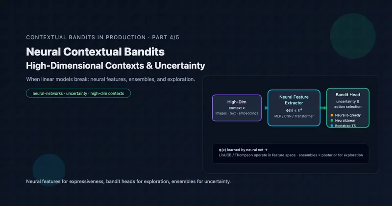
- Part 4 Neural Contextual Bandits for High-Dimensional Data
- Part 5 Deploying Contextual Bandits: Production Guide and Offline Evaluation


