Neural Contextual Bandits for High-Dimensional Data
Part 4 of 5: When Linear Models Aren’t Enough
TL;DR: Neural contextual bandits handle high-dimensional contexts (images, text) and complex nonlinear reward functions that linear models can’t capture. The key challenge is uncertainty quantification—neural networks don’t naturally provide confidence bounds. We solve this with bootstrap ensembles (approximating posteriors) and hybrid approaches like NeuralLinear (neural features + LinUCB). This post provides complete implementations and guidance on when the complexity is worth it.
Reading time: ~22 minutes
Introduction: When Linear Models Break
Parts 1-3 covered the foundations and core algorithms. LinUCB and Linear Thompson Sampling work great when rewards are approximately linear in features:
But what if:
- Rewards are highly nonlinear? Complex interactions between features that linear models can’t capture
- Contexts are high-dimensional raw inputs? Images (100k+ pixels), text (embedding dimensions), audio
- You have complex feature interactions? Product of features, higher-order terms
Linear models fail. You need neural networks.
But neural networks introduce a critical challenge: how do we explore?
- LinUCB uses confidence bounds:
- Thompson Sampling uses posteriors:
- Neural networks give point predictions: with no uncertainty
This post solves the uncertainty problem with three approaches:
- Neural ε-greedy: Simplest baseline (random exploration)
- NeuralLinear: Neural features + LinUCB (best of both worlds)
- Bootstrap Thompson Sampling: Ensemble for uncertainty quantification
Plus handling high-dimensional action spaces (thousands to millions of actions).
When to Use Neural Contextual Bandits
Decision Framework
Use Neural Bandits When:
✅ High-dimensional raw inputs:
- Images (product photos, user-generated content)
- Text (article content, user reviews)
- Audio (podcast clips, voice commands)
- Video (thumbnails, short clips)
✅ Complex nonlinear reward functions:
- Deep feature interactions that linear models miss
- Tried feature engineering, still underfitting
- Domain experts say “relationships are definitely nonlinear”
✅ Sufficient training data:
- Need 10-100x more data than linear models
- Typically 10k+ interactions minimum
- More for complex architectures
Stick with Linear When:
❌ You can engineer good features:
- Domain knowledge suggests which features matter
- Embeddings from pretrained models work well
- Linear model achieves reasonable performance
❌ Limited training data:
- <1000 interactions per action
- Linear models more sample-efficient
❌ Need interpretability:
- Must explain why actions were chosen
- Regulatory requirements for transparency
❌ Computational constraints:
- Neural inference is 10-100x slower
- Training is much more expensive
The Uncertainty Problem: Why Neural Bandits Are Hard
The Challenge
Linear models give us uncertainty for free:
LinUCB: Confidence ellipsoid from covariance matrix
Linear Thompson: Posterior from Bayesian updates
Neural networks: Just a point estimate with no uncertainty 😞
Why Uncertainty Matters
Without uncertainty, we can’t explore intelligently:
# Bad: Neural network without uncertainty
neural_net = train_neural_network(data)

for context in contexts:
    # Get predictions for all actions
    q_values = neural_net.predict(context)  # Just point estimates

    # No way to know which estimates are uncertain!
    # Can only do pure exploitation (greedy) or random exploration (ε-greedy)
    action = argmax(q_values)  # Greedy
Problem: Novel contexts (far from training data) get confident predictions that might be wrong. We need to know “I’m uncertain about action A in this context.”
Three Solutions
| Approach | How It Works | Pros | Cons |
|---|---|---|---|
| Neural ε-greedy | Random exploration | Simple, works | Inefficient (wastes exploration) |
| NeuralLinear | Neural features + LinUCB | Directed exploration, interpretable | Assumes linear in learned features |
| Bootstrap Ensemble | Multiple networks, disagreement = uncertainty | Flexible, approximates Bayesian | Expensive (10x networks) |
Let’s implement all three.
Neural ε-greedy: The Simplest Baseline
When you can’t quantify uncertainty, fall back to random exploration.
Architecture
Implementation
import torch
import torch.nn as nn
import torch.optim as optim
import numpy as np
from collections import deque
import random

class NeuralEpsilonGreedy:
    """
    Neural network with ε-greedy exploration.

    Uses deep Q-learning: network predicts Q-value (expected reward)
    for each action given context. Explores randomly with probability ε.
    """
    def __init__(self, n_features, n_actions,
                 hidden_dims=[256, 128], epsilon=0.1,
                 lr=1e-3, buffer_size=10000, batch_size=32):
        """
        Args:
            n_features: Input dimensionality
            n_actions: Number of actions
            hidden_dims: Hidden layer sizes
            epsilon: Exploration probability
            lr: Learning rate
            buffer_size: Experience replay buffer size
            batch_size: Minibatch size for training
        """
        self.n_actions = n_actions
        self.epsilon = epsilon
        self.batch_size = batch_size

        # Build neural network
        layers = []
        prev_dim = n_features
        for hidden_dim in hidden_dims:
            layers.append(nn.Linear(prev_dim, hidden_dim))
            layers.append(nn.ReLU())
            prev_dim = hidden_dim
        layers.append(nn.Linear(prev_dim, n_actions))

        self.model = nn.Sequential(*layers)
        self.optimizer = optim.Adam(self.model.parameters(), lr=lr)
        self.criterion = nn.MSELoss()

        # Experience replay buffer: (context, action, reward)
        self.buffer = deque(maxlen=buffer_size)

    def select_action(self, context):
        """
        ε-greedy action selection.

        Args:
            context: Feature vector (numpy array)

        Returns:
            action: Chosen action index
        """
        if np.random.random() < self.epsilon:
            # Explore: random action
            return np.random.randint(self.n_actions)

        # Exploit: best action according to Q-network
        with torch.no_grad():
            context_tensor = torch.FloatTensor(context).unsqueeze(0)
            q_values = self.model(context_tensor)
            return torch.argmax(q_values).item()

    def update(self, context, action, reward):
        """
        Store experience and train network.

        Args:
            context: Observed context
            action: Action taken
            reward: Reward received
        """
        # Store in replay buffer
        self.buffer.append((context, action, reward))

        # Train on minibatch if enough data
        if len(self.buffer) >= self.batch_size:
            self._train_step()

    def _train_step(self):
        """Train network on random minibatch from buffer."""
        # Sample minibatch
        batch = random.sample(self.buffer, self.batch_size)
        contexts, actions, rewards = zip(*batch)

        # Convert to tensors
        context_tensor = torch.FloatTensor(contexts)
        action_tensor = torch.LongTensor(actions)
        reward_tensor = torch.FloatTensor(rewards)

        # Forward pass: predict Q-values
        q_values = self.model(context_tensor)

        # Extract Q-values for taken actions
        q_values_selected = q_values.gather(1, action_tensor.unsqueeze(1)).squeeze()

        # Loss: MSE between predicted Q and observed reward
        loss = self.criterion(q_values_selected, reward_tensor)

        # Backprop
        self.optimizer.zero_grad()
        loss.backward()
        self.optimizer.step()

    def get_q_values(self, context):
        """Get Q-values for all actions (for debugging)."""
        with torch.no_grad():
            context_tensor = torch.FloatTensor(context).unsqueeze(0)
            return self.model(context_tensor).squeeze().numpy()


# Example usage
if __name__ == "__main__":
    # High-dimensional context (e.g., image embedding)
    n_features = 512
    n_actions = 10

    bandit = NeuralEpsilonGreedy(
        n_features=n_features,
        n_actions=n_actions,
        hidden_dims=[256, 128],
        epsilon=0.1,
        lr=1e-3
    )

    # Simulate training
    for t in range(1000):
        context = np.random.randn(n_features)  # Random context
        action = bandit.select_action(context)

        # Simulate reward (true reward = sum of context, varies by action)
        true_reward = (action / n_actions) * np.sum(context[:10])
        noise = np.random.normal(0, 0.1)
        reward = true_reward + noise

        bandit.update(context, action, reward)

        if t % 100 == 0:
            print(f"Round {t}: Action {action}, Reward {reward:.3f}")
When to Use Neural ε-greedy
✅ Use as baseline when:
- First trying neural bandits (validate infrastructure)
- High-dimensional contexts (images, text)
- Simple to implement and explain
❌ Limitations:
- Random exploration (inefficient)
- No directed exploration toward uncertainty
- Still O(T^(2/3)) regret (suboptimal)
Production tip: Start here, then upgrade to NeuralLinear or Bootstrap if you need better sample efficiency.
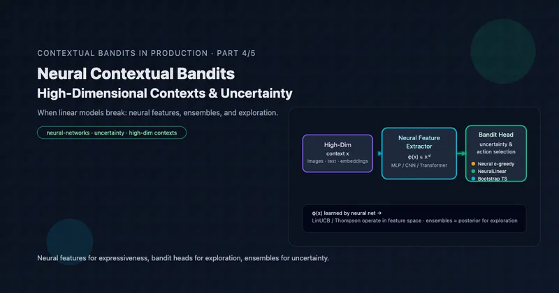
NeuralLinear: Best of Both Worlds
Key insight: Use neural network to learn good features, then apply LinUCB in the learned feature space.
Architecture
Why This Works
- Neural network learns good representations φ(x) from raw inputs
- LinUCB operates in feature space, providing confidence bounds
- Best of both: Neural expressiveness + principled exploration
Assumption: Rewards are linear in learned features φ(x), even if nonlinear in raw context x.
Implementation
class NeuralLinear:
    """
    Neural feature extractor + LinUCB.

    Neural network learns representation φ(x), then LinUCB operates
    in this learned feature space with confidence-based exploration.
    """
    def __init__(self, n_actions, input_dim, feature_dim=128,
                 hidden_dims=[256, 128], alpha=1.0, lambda_=1.0):
        """
        Args:
            n_actions: Number of actions
            input_dim: Raw context dimensionality
            feature_dim: Learned feature dimensionality
            hidden_dims: Hidden layer sizes for feature extractor
            alpha: LinUCB exploration parameter
            lambda_: LinUCB regularization parameter
        """
        self.n_actions = n_actions
        self.feature_dim = feature_dim
        self.alpha = alpha
        self.lambda_ = lambda_

        # Neural feature extractor
        layers = []
        prev_dim = input_dim
        for hidden_dim in hidden_dims:
            layers.append(nn.Linear(prev_dim, hidden_dim))
            layers.append(nn.ReLU())
            prev_dim = hidden_dim
        layers.append(nn.Linear(prev_dim, feature_dim))
        layers.append(nn.ReLU())  # Ensure positive features

        self.feature_model = nn.Sequential(*layers)
        self.optimizer = optim.Adam(self.feature_model.parameters(), lr=1e-3)

        # LinUCB in learned feature space
        self.A = [lambda_ * np.eye(feature_dim) for _ in range(n_actions)]
        self.b = [np.zeros(feature_dim) for _ in range(n_actions)]

        # Training buffer
        self.buffer = deque(maxlen=10000)

    def extract_features(self, context):
        """
        Extract features using neural network.

        Args:
            context: Raw context (numpy array)

        Returns:
            features: Learned representation φ(x)
        """
        with torch.no_grad():
            context_tensor = torch.FloatTensor(context).unsqueeze(0)
            features = self.feature_model(context_tensor).squeeze().numpy()
        return features

    def select_action(self, context):
        """
        Select action with highest UCB in learned feature space.

        Args:
            context: Raw context

        Returns:
            action: Chosen action index
        """
        # Extract features
        features = self.extract_features(context)
        features = features.reshape(-1, 1)  # Column vector

        # Compute UCB for each action (same as LinUCB)
        ucb_values = np.zeros(self.n_actions)
        for a in range(self.n_actions):
            A_inv = np.linalg.inv(self.A[a])
            theta = A_inv @ self.b[a]

            predicted_reward = theta.T @ features
            confidence_bonus = self.alpha * np.sqrt(features.T @ A_inv @ features)

            ucb_values[a] = predicted_reward + confidence_bonus

        return np.argmax(ucb_values)

    def update(self, context, action, reward):
        """
        Update LinUCB estimates and (optionally) train feature extractor.

        Args:
            context: Raw context
            action: Action taken
            reward: Reward received
        """
        # Extract features
        features = self.extract_features(context)
        features = features.reshape(-1, 1)

        # Update LinUCB (same as before)
        self.A[action] += features @ features.T
        self.b[action] += reward * features.squeeze()

        # Store for feature learning
        self.buffer.append((context, action, reward))

        # Periodically update feature extractor
        if len(self.buffer) >= 32 and len(self.buffer) % 10 == 0:
            self._train_features()

    def _train_features(self):
        """
        Train feature extractor to predict rewards.

        This is optional but can improve feature quality over time.
        """
        if len(self.buffer) < 32:
            return

        # Sample minibatch
        batch = random.sample(self.buffer, 32)
        contexts, actions, rewards = zip(*batch)

        # Extract features
        context_tensor = torch.FloatTensor(contexts)
        features = self.feature_model(context_tensor)

        # Predict rewards using current LinUCB parameters
        predicted_rewards = []
        for i, a in enumerate(actions):
            A_inv = np.linalg.inv(self.A[a])
            theta = A_inv @ self.b[a]
            pred = theta.T @ features[i].detach().numpy()
            predicted_rewards.append(pred)

        predicted_tensor = torch.FloatTensor(predicted_rewards)
        reward_tensor = torch.FloatTensor(rewards)

        # Train to predict rewards better
        loss = nn.MSELoss()(predicted_tensor, reward_tensor)

        self.optimizer.zero_grad()
        loss.backward()
        self.optimizer.step()

    def get_theta(self, action):
        """Get learned LinUCB parameters for an action."""
        A_inv = np.linalg.inv(self.A[action])
        return A_inv @ self.b[action]


# Example usage
if __name__ == "__main__":
    # Image-like context (e.g., 28x28 = 784 pixels)
    input_dim = 784
    n_actions = 10

    bandit = NeuralLinear(
        n_actions=n_actions,
        input_dim=input_dim,
        feature_dim=64,  # Compress to 64-dim
        hidden_dims=[256, 128],
        alpha=1.0,
        lambda_=1.0
    )

    for t in range(1000):
        context = np.random.randn(input_dim)
        action = bandit.select_action(context)

        # Simulate reward
        reward = (action / n_actions) * np.sum(context[:10]) + np.random.normal(0, 0.1)

        bandit.update(context, action, reward)

        if t % 100 == 0:
            print(f"Round {t}: Action {action}, Reward {reward:.3f}")
            print(f"  Feature norm: {np.linalg.norm(bandit.extract_features(context)):.3f}")
When to Use NeuralLinear
✅ Use when:
- High-dimensional raw contexts (images, text)
- Rewards are linear in good features (but you don’t know what features)
- Want directed exploration (better than ε-greedy)
- Need some interpretability (can examine θ weights)
✅ Advantages:
- Confidence bounds guide exploration
- More sample-efficient than neural ε-greedy
- Can inspect learned features and weights
❌ Limitations:
- Assumes linearity in learned features
- Training feature extractor adds complexity
- Not as flexible as full neural Thompson Sampling
Bootstrap Thompson Sampling: Ensemble for Uncertainty
Core idea: Train an ensemble of neural networks on bootstrap samples. Disagreement between networks = uncertainty.
Why Ensembles Approximate Bayesian Posteriors
Bayesian Thompson Sampling:
- Posterior:
- Sample:
- Choose:
Bootstrap approximation:
- Train K networks on different bootstrap samples
- Each network approximates a sample from posterior
- Sample random network
- Choose:
Intuition: In regions with lots of data, all networks agree (low uncertainty). In novel regions, networks disagree (high uncertainty) → naturally explores.
Implementation
class BootstrappedNeuralBandit:
    """
    Bootstrap ensemble for Thompson Sampling approximation.

    Trains K neural networks on bootstrap samples of data.
    Action selection: randomly pick one network, use its predictions.
    Disagreement between networks indicates uncertainty.
    """
    def __init__(self, n_features, n_actions, n_models=10,
                 hidden_dims=[256, 128], lr=1e-3,
                 buffer_size=10000, batch_size=32):
        """
        Args:
            n_features: Input dimensionality
            n_actions: Number of actions
            n_models: Number of networks in ensemble
            hidden_dims: Hidden layer sizes
            lr: Learning rate
            buffer_size: Replay buffer size
            batch_size: Minibatch size
        """
        self.n_models = n_models
        self.n_actions = n_actions
        self.batch_size = batch_size

        # Create ensemble of neural networks
        self.models = []
        self.optimizers = []

        for _ in range(n_models):
            # Build network
            layers = []
            prev_dim = n_features
            for hidden_dim in hidden_dims:
                layers.append(nn.Linear(prev_dim, hidden_dim))
                layers.append(nn.ReLU())
                prev_dim = hidden_dim
            layers.append(nn.Linear(prev_dim, n_actions))

            model = nn.Sequential(*layers)
            optimizer = optim.Adam(model.parameters(), lr=lr)

            self.models.append(model)
            self.optimizers.append(optimizer)

        self.criterion = nn.MSELoss()
        self.buffer = deque(maxlen=buffer_size)

    def select_action(self, context):
        """
        Thompson Sampling style: sample one network, use its predictions.

        Args:
            context: Feature vector

        Returns:
            action: Chosen action index
        """
        # Randomly sample one model from ensemble (Thompson Sampling)
        model_idx = np.random.randint(self.n_models)

        with torch.no_grad():
            context_tensor = torch.FloatTensor(context).unsqueeze(0)
            q_values = self.models[model_idx](context_tensor)
            return torch.argmax(q_values).item()

    def update(self, context, action, reward):
        """
        Store experience and train all networks on bootstrap samples.

        Args:
            context: Observed context
            action: Action taken
            reward: Reward received
        """
        # Store in buffer
        self.buffer.append((context, action, reward))

        # Train each model on a bootstrap sample
        if len(self.buffer) >= self.batch_size:
            self._train_step()

    def _train_step(self):
        """Train each model on a different bootstrap sample."""
        for k in range(self.n_models):
            # Bootstrap: resample with replacement
            bootstrap_batch = random.choices(self.buffer, k=self.batch_size)
            contexts, actions, rewards = zip(*bootstrap_batch)

            # Convert to tensors
            context_tensor = torch.FloatTensor(contexts)
            action_tensor = torch.LongTensor(actions)
            reward_tensor = torch.FloatTensor(rewards)

            # Forward pass
            q_values = self.models[k](context_tensor)
            q_selected = q_values.gather(1, action_tensor.unsqueeze(1)).squeeze()

            # Loss
            loss = self.criterion(q_selected, reward_tensor)

            # Backprop
            self.optimizers[k].zero_grad()
            loss.backward()
            self.optimizers[k].step()

    def get_uncertainty(self, context):
        """
        Compute uncertainty as disagreement between models.

        Args:
            context: Feature vector

        Returns:
            mean: Mean Q-values across ensemble
            std: Standard deviation (uncertainty measure)
        """
        with torch.no_grad():
            context_tensor = torch.FloatTensor(context).unsqueeze(0)

            # Get predictions from all models
            predictions = []
            for model in self.models:
                q_values = model(context_tensor).squeeze().numpy()
                predictions.append(q_values)

            predictions = np.array(predictions)  # Shape: [n_models, n_actions]

            mean = predictions.mean(axis=0)
            std = predictions.std(axis=0)

            return mean, std


# Example usage with uncertainty visualization
if __name__ == "__main__":
    n_features = 512
    n_actions = 10
    n_models = 10

    bandit = BootstrappedNeuralBandit(
        n_features=n_features,
        n_actions=n_actions,
        n_models=n_models,
        hidden_dims=[256, 128],
        lr=1e-3
    )

    for t in range(2000):
        context = np.random.randn(n_features)
        action = bandit.select_action(context)

        # Simulate reward
        true_reward = (action / n_actions) * np.sum(context[:10])
        noise = np.random.normal(0, 0.1)
        reward = true_reward + noise

        bandit.update(context, action, reward)

        if t % 200 == 0:
            mean, std = bandit.get_uncertainty(context)
            print(f"\nRound {t}:")
            print(f"  Chosen action: {action}, Reward: {reward:.3f}")
            print(f"  Uncertainty (avg std): {std.mean():.3f}")
            print(f"  Action {action} uncertainty: {std[action]:.3f}")
When to Use Bootstrap Thompson Sampling
✅ Use when:
- Need best sample efficiency (Thompson Sampling properties)
- Can afford computational cost (K networks, K forward passes)
- Want uncertainty quantification (ensemble disagreement)
- Don’t need interpretability
✅ Advantages:
- Approximates Bayesian Thompson Sampling
- Natural exploration-exploitation balance
- Often best empirical performance
❌ Limitations:
- Expensive: K times the cost (typically K = 5-20)
- No theoretical guarantees (approximate Thompson)
- Less interpretable than NeuralLinear
Ensemble Size Tuning
| n_models | Computational Cost | Uncertainty Quality | When to Use |
|---|---|---|---|
| 3-5 | Low (3-5x) | Rough approximation | Quick prototyping |
| 10 | Medium (10x) | Good uncertainty | Production default |
| 20 | High (20x) | Best uncertainty | Critical applications |
Diminishing returns: Beyond 10-15 models, improvement is marginal.
High-Dimensional Action Spaces
Problem: With thousands to millions of actions (e.g., all products in catalog), standard bandits don’t scale.
- Can’t maintain separate parameters for each action
- Can’t explore all actions
- Need generalization across actions
Solution 1: Action Embeddings
Idea: Represent actions in low-dimensional space. Learn that similar actions have similar rewards.
class ActionEmbeddingBandit:
    """
    Contextual bandit with action embeddings.

    Instead of learning separate parameters for each action,
    learns reward as function of (context, action_embedding).
    Enables generalization across similar actions.
    """
    def __init__(self, context_dim, action_embedding_dim,
                 hidden_dims=[256, 128], lr=1e-3):
        """
        Args:
            context_dim: Context feature dimensionality
            action_embedding_dim: Action embedding dimensionality
            hidden_dims: Hidden layer sizes
            lr: Learning rate
        """
        self.action_embedding_dim = action_embedding_dim

        # Neural network: (context, action_embedding) → reward
        input_dim = context_dim + action_embedding_dim

        layers = []
        prev_dim = input_dim
        for hidden_dim in hidden_dims:
            layers.append(nn.Linear(prev_dim, hidden_dim))
            layers.append(nn.ReLU())
            prev_dim = hidden_dim
        layers.append(nn.Linear(prev_dim, 1))  # Scalar reward prediction

        self.model = nn.Sequential(*layers)
        self.optimizer = optim.Adam(self.model.parameters(), lr=lr)
        self.criterion = nn.MSELoss()

        self.buffer = deque(maxlen=10000)

    def select_action(self, context, candidate_actions, action_embeddings):
        """
        Select action from candidates using learned reward function.

        Args:
            context: User/situation features
            candidate_actions: List of action IDs to choose from
            action_embeddings: Dict mapping action_id → embedding vector

        Returns:
            action: Chosen action ID
        """
        scores = []

        with torch.no_grad():
            context_tensor = torch.FloatTensor(context)

            for action_id in candidate_actions:
                # Get action embedding
                action_emb = action_embeddings[action_id]
                action_tensor = torch.FloatTensor(action_emb)

                # Concatenate context + action embedding
                combined = torch.cat([context_tensor, action_tensor])

                # Predict reward
                reward_pred = self.model(combined.unsqueeze(0)).item()
                scores.append(reward_pred)

        # Choose action with highest predicted reward
        # (could add exploration here with ε-greedy or UCB)
        best_idx = np.argmax(scores)
        return candidate_actions[best_idx]

    def update(self, context, action_embedding, reward):
        """
        Update model based on observed reward.

        Args:
            context: Context features
            action_embedding: Embedding of chosen action
            reward: Observed reward
        """
        self.buffer.append((context, action_embedding, reward))

        if len(self.buffer) >= 32:
            self._train_step()

    def _train_step(self):
        """Train on minibatch."""
        batch = random.sample(self.buffer, 32)
        contexts, action_embs, rewards = zip(*batch)

        # Concatenate context + action embeddings
        combined = []
        for ctx, act_emb in zip(contexts, action_embs):
            combined.append(np.concatenate([ctx, act_emb]))

        combined_tensor = torch.FloatTensor(combined)
        reward_tensor = torch.FloatTensor(rewards).unsqueeze(1)

        # Forward pass
        predictions = self.model(combined_tensor)
        loss = self.criterion(predictions, reward_tensor)

        # Backprop
        self.optimizer.zero_grad()
        loss.backward()
        self.optimizer.step()


# Example: E-commerce with product embeddings
if __name__ == "__main__":
    # Simulate product catalog
    n_products = 10000
    context_dim = 50  # User features
    embedding_dim = 64  # Product embeddings

    # Generate product embeddings (in practice, from item2vec, product features, etc.)
    product_embeddings = {
        product_id: np.random.randn(embedding_dim)
        for product_id in range(n_products)
    }

    bandit = ActionEmbeddingBandit(
        context_dim=context_dim,
        action_embedding_dim=embedding_dim,
        hidden_dims=[256, 128]
    )

    for t in range(1000):
        # User context
        context = np.random.randn(context_dim)

        # Candidate products (e.g., from retrieval stage)
        candidates = random.sample(range(n_products), 100)

        # Select product
        chosen_product = bandit.select_action(context, candidates, product_embeddings)

        # Simulate reward
        reward = np.random.random()  # In practice: purchase, click, etc.

        # Update
        action_emb = product_embeddings[chosen_product]
        bandit.update(context, action_emb, reward)

        if t % 100 == 0:
            print(f"Round {t}: Chose product {chosen_product}, Reward: {reward:.3f}")
Solution 2: Two-Stage Selection
Idea: First, narrow to top-K candidates (fast heuristic). Then, run bandit on top-K.
def two_stage_selection(context, all_actions, bandit, K=100):
    """
    Two-stage action selection for large action spaces.

    Stage 1: Fast filtering to top-K candidates
    Stage 2: Bandit selection from candidates

    Args:
        context: User/situation features
        all_actions: Full action space (large)
        bandit: Bandit algorithm instance
        K: Number of candidates to keep

    Returns:
        action: Final selected action
    """
    # Stage 1: Fast filtering (e.g., dot product with user embedding)
    user_embedding = context[:64]  # First 64 dims

    scores = []
    for action in all_actions:
        # Fast heuristic: dot product similarity
        action_embedding = get_action_embedding(action)
        score = np.dot(user_embedding, action_embedding)
        scores.append((score, action))

    # Keep top K
    scores.sort(reverse=True)
    candidates = [action for _, action in scores[:K]]

    # Stage 2: Bandit selects from candidates
    action = bandit.select_action(context, candidates)

    return action
Tradeoff: Speed vs optimality. Fast heuristic might filter out good actions, but makes bandits tractable.
Algorithm Comparison for Neural Bandits
Performance vs Complexity
Detailed Comparison
| Algorithm | Exploration | Computational Cost | Sample Efficiency | When to Use |
|---|---|---|---|---|
| Neural ε-greedy | Random | 1x (baseline) | Low | Simple baseline, quick start |
| NeuralLinear | Confidence bounds | 1.5x (feature extraction) | Medium | Want interpretability + efficiency |
| Bootstrap TS | Ensemble disagreement | 10-20x (K networks) | High | Need best performance, have compute |
| Action Embeddings | Depends on base | 1x | Medium | High-dim action spaces (1000s+) |
Key Takeaways
Essential concepts:
Use neural bandits when linear models fail:
- High-dimensional raw inputs (images, text, audio)
- Complex nonlinear reward functions
- But need 10-100x more data than linear models
Uncertainty quantification is the key challenge:
- Neural networks give point estimates, not uncertainty
- Need uncertainty to explore intelligently
- Three solutions: ε-greedy (random), NeuralLinear (features), Bootstrap (ensemble)
NeuralLinear is often the best starting point:
- Neural features + LinUCB confidence bounds
- Directed exploration (better than random)
- Some interpretability (examine θ weights)
Bootstrap Thompson Sampling for maximum performance:
- Trains K networks on bootstrap samples
- Disagreement = uncertainty
- Best sample efficiency, but K times the cost
High-dimensional action spaces need special handling:
- Action embeddings (generalize across similar actions)
- Two-stage selection (filter then select)
- Can’t maintain separate parameters for millions of actions
Practical recommendations:
| Your Situation | Recommended Approach |
|---|---|
| Quick prototype | Neural ε-greedy (simplest) |
| Production baseline | NeuralLinear (balanced) |
| Maximum performance | Bootstrap TS with 10 networks |
| >1000 actions | Action embeddings or two-stage |
| Limited compute | NeuralLinear or ε-greedy |
| Need interpretability | NeuralLinear (can inspect θ) |
Common pitfalls to avoid:
❌ Using neural bandits when linear suffices (overfitting, sample inefficiency)
❌ Forgetting to normalize features (neural networks are sensitive)
❌ Too few bootstrap models (K < 5 gives poor uncertainty)
❌ Too many bootstrap models (K > 20 diminishing returns)
❌ Not maintaining replay buffer (catastrophic forgetting)
Further Reading
Neural bandit papers:
- Deep Bayesian Bandits Showdown (Riquelme et al., 2018) - Comprehensive comparison of neural methods. ICLR 2018
- Neural Contextual Bandits with UCB (Zhou et al., 2020) - NeuralUCB algorithm. ICML 2020
- Deep Exploration via Bootstrapped DQN (Osband et al., 2016) - Bootstrap for deep RL/bandits. NeurIPS 2016
Code repositories:
- TensorFlow Agents: Neural bandit implementations
- RecoGym: Recommendation environment for testing neural bandits
Blog posts:
Article series
Adaptive Optimization at Scale: Contextual Bandits from Theory to Production
- Part 1 When to Use Contextual Bandits: The Decision Framework
- Part 2 Contextual Bandit Theory: Regret Bounds and Exploration
- Part 3 Implementing Contextual Bandits: Complete Algorithm Guide
- Part 4 Neural Contextual Bandits for High-Dimensional Data
- Part 5 Deploying Contextual Bandits: Production Guide and Offline Evaluation