PPO for Language Models: The RLHF Workhorse

Part 2 of 5: The Industry Standard

Updated 31 Oct 2026: The clipping section now covers all four cases, not two. Corrected the 7B memory numbers: PPO’s four models need about 252 GB with mixed-precision Adam, not 84 GB. Fixed the sign of the KL-in-the-loss formula, and moved the π_old update in the pseudocode outside the epoch loop. The PyTorch trainer now masks padding, puts the reward on the EOS token, uses a real value head, applies the entropy bonus, and runs minibatches. Series labels now count five parts.

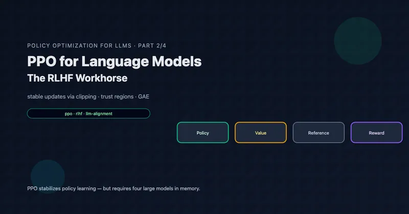
TL;DR: PPO (Proximal Policy Optimization) is the algorithm the classic RLHF recipe was built on: it trained InstructGPT (Ouyang et al., 2022) and Anthropic’s 2022 RLHF assistant (Bai et al., 2022). It provides stable training through clipped objectives and flexible advantage estimation via GAE. But this comes at a cost: four models (policy, reference, value, reward) straining GPU memory. Understanding PPO deeply reveals why simpler alternatives like GRPO emerged.

Reading time: ~28 minutes

Prerequisites: Part 1: RL Foundations covers policy gradients, value functions, and advantage estimation. Symbols follow the series notation.

From REINFORCE to PPO

In Part 1, we saw that policy gradients are powerful but suffer from high variance. Actor-critic methods add a value function to reduce variance, but introduce their own challenges: training two networks that must improve together without destabilizing each other.

PPO (Proximal Policy Optimization) addresses stability through a deceptively simple idea: limit how much the policy can change in a single update. If updates are small enough, the value function doesn’t become stale, and training remains stable.

But “small updates” is vague. How do we formalize it? And how do we enforce it efficiently?

The Trust Region Idea

The Problem with Large Updates

Consider what happens when we take a policy gradient step:

1. Collect trajectories using current policy $\pi_{\theta_{\text{old}}}$
2. Compute advantages using value function $V_\psi$
3. Update: $\theta \leftarrow \theta + \alpha \nabla_\theta J(\theta)$

The problem: our advantages were computed for $\pi_{\theta_{\text{old}}}$, but we’re evaluating actions under $\pi_\theta$. If $\theta$ changes too much, the advantages become stale—they no longer reflect the true quality of actions under the new policy.

This can cause:

• Overshooting: A good action gets reinforced too strongly
• Policy collapse: All probability mass shifts to one action
• Training instability: Performance oscillates wildly

Trust Regions: The Concept

A trust region is a constraint on how much the policy can change:

where $D$ is some distance measure between policies, and $\delta$ is a small threshold.

Within the trust region, our local approximation (using old advantages) is valid. Outside it, we can’t trust our gradient estimates.

TRPO: The Principled Approach

Trust Region Policy Optimization (TRPO) uses KL divergence as the distance:

TRPO solves this constrained optimization using second-order methods (conjugate gradient + line search). It’s theoretically elegant but:

• Computationally expensive
• Complex to implement
• Hard to parallelize

This motivated PPO: can we get trust region benefits with first-order methods?

From TRPO to PPO: The Clipped Objective

PPO’s insight: instead of enforcing a hard constraint, clip the objective so that updates beyond the trust region give no additional benefit.

The Importance Sampling Ratio

First, we rewrite the policy gradient using importance sampling:

Define the importance ratio:

When $\theta = \theta_{\text{old}}$, we have $\rho = 1$. As $\theta$ diverges from $\theta_{\text{old}}$, $\rho$ moves away from 1.

The Clipped Surrogate Objective

PPO’s objective clips the ratio to prevent large updates:

Let’s unpack this carefully.

How Clipping Works

The min takes the smaller of the unclipped term $\rho_t \hat{A}_t$ and the clipped term. Which one wins depends on the sign of the advantage and on where the ratio sits. There are four cases:

Rows 2 and 4 are the familiar ones. The ratio has moved the favoured way — probability up for a good action, down for a bad one — by more than $\varepsilon$. The clipped term is a constant, so the gradient switches off: that’s enough for this batch.

Rows 1 and 3 are where the min earns its place. Here the ratio has moved the unfavoured way: a good action became less likely ($\rho_t < 1-\varepsilon$), or a bad action more likely ($\rho_t > 1+\varepsilon$). Clipping alone would flatten the objective and stop the correction. The min keeps the unclipped term instead, so the gradient stays on and pulls the ratio back. For a bad action, the penalty $\rho_t \hat{A}_t$ keeps growing with $\rho_t$, and nothing caps it.

The “Pessimistic” Bound

The $\min$ in the objective creates a pessimistic bound: we take the worse of (unclipped, clipped) for each term.

The objective never rewards moving more than $\varepsilon$ in the favoured direction, but keeps penalising moves in the unfavoured direction without limit.

This is conservative by design—it prevents the optimizer from exploiting stale advantages.

Why $\varepsilon = 0.2$?

The canonical choice is $\varepsilon = 0.2$. Clipping removes the gradient once the ratio leaves $[0.8, 1.2]$ in the favoured direction. It doesn’t cap the ratio itself, which can overshoot: parameters are shared across tokens, so a step taken for one token moves the others too, and several minibatch steps run on each batch. Empirically, 0.2 balances stability and learning speed. Some implementations use 0.1 for more conservative updates.

Key Insight: PPO’s clipping creates a “soft trust region” using only first-order optimization. The policy can change, but changes beyond $\varepsilon$ provide no additional gradient signal. It’s not a hard constraint, but it works remarkably well in practice.

Generalized Advantage Estimation (GAE)

PPO pairs the clipped objective with Generalized Advantage Estimation (GAE), a flexible way to estimate advantages.

The Bias-Variance Tradeoff

Recall from Part 1 that we can estimate advantages in different ways:

Monte Carlo (MC): $\hat{A}_t^{\text{MC}} = G_t - V(s_t) = \sum_{k=0}^{T-t} \gamma^k r_{t+k} - V(s_t)$

• Unbiased: Uses actual returns
• High variance: Includes all future randomness

Temporal Difference (TD): $\hat{A}_t^{\text{TD}} = r_t + \gamma V(s_{t+1}) - V(s_t) = \delta_t$

• Biased: Uses estimated $V(s_{t+1})$ instead of true expected return
• Low variance: Only one step of randomness

GAE: Interpolating Between MC and TD

GAE introduces parameter $\lambda \in [0, 1]$ to interpolate:

where $\delta_t = r_t + \gamma V(s_{t+1}) - V(s_t)$ is the TD error.

Special cases:

• $\lambda = 0$: $\hat{A}_t = \delta_t$ (TD, low variance, high bias)
• $\lambda = 1$: $\hat{A}_t = \sum_k \gamma^k \delta_{t+k} = G_t - V(s_t)$ (MC, high variance, low bias)

Practical Computation

GAE can be computed efficiently backwards through the trajectory:

Starting from the end of the episode ($\hat{A}_T = 0$ or $\hat{A}_T = \delta_T$), we recurse backwards.

def compute_gae(rewards, values, gamma=0.99, lam=0.95):
    """
    Compute GAE advantages.
    
    Args:
        rewards: [T] rewards at each timestep
        values: [T+1] value estimates (includes bootstrap V(s_T+1))
        gamma: Discount factor
        lam: GAE lambda parameter
    
    Returns:
        advantages: [T] GAE advantage estimates
    """
    T = len(rewards)
    advantages = torch.zeros(T)
    last_adv = 0
    
    for t in reversed(range(T)):
        # TD error: δ_t = r_t + γV(s_{t+1}) - V(s_t)
        delta = rewards[t] + gamma * values[t + 1] - values[t]
        # GAE recursion: A_t = δ_t + γλ A_{t+1}
        advantages[t] = delta + gamma * lam * last_adv
        last_adv = advantages[t]
    
    return advantages

Choosing $\lambda$

The default $\lambda = 0.95$ works well across many domains, including LLM fine-tuning.

Key Insight: GAE lets us tune the bias-variance tradeoff. High $\lambda$ trusts actual returns more; low $\lambda$ trusts the value function more. For LLMs with sparse rewards, higher $\lambda$ is often better since the value function may be inaccurate at intermediate states. Ahmadian et al. (2024) found the same in RLHF: leaning on the value function (low $\lambda$) performed worse, and they argue for dropping the critic altogether — the starting point of Part 3.

The Complete PPO Algorithm

Now let’s put it all together.

PPO-Clip Algorithm

Algorithm: PPO-Clip

Hyperparameters: 
    ε (clip ratio, typically 0.2)
    γ (discount, typically 0.99 or 1.0)
    λ (GAE lambda, typically 0.95)
    K (epochs per batch, typically 3-10)
    M (minibatch size)

Initialize: Policy π_θ, Value function V_ψ

For iteration = 1, 2, ...:
    ┌─────────────────────────────────────────────────────┐
    │ Phase 1: Collect Experience                         │
    │ ─────────────────────────────────────────────────── │
    │ Run π_θ for T timesteps, collecting:                │
    │   {s_t, a_t, r_t, s_{t+1}} for t = 1...T           │
    │                                                     │
    │ Compute value estimates V_ψ(s_t) for all t          │
    └─────────────────────────────────────────────────────┘
    
    ┌─────────────────────────────────────────────────────┐
    │ Phase 2: Compute Advantages                         │
    │ ─────────────────────────────────────────────────── │
    │ For t = T-1 down to 0:                              │
    │     δ_t = r_t + γV_ψ(s_{t+1}) - V_ψ(s_t)           │
    │     Â_t = δ_t + γλ Â_{t+1}    (GAE)                │
    │                                                     │
    │ Compute returns: R̂_t = Â_t + V_ψ(s_t)              │
    └─────────────────────────────────────────────────────┘
    
    ┌─────────────────────────────────────────────────────┐
    │ Phase 3: Optimization (K epochs)                    │
    │ ─────────────────────────────────────────────────── │
    │ For epoch = 1 to K:                                 │
    │     For each minibatch of size M:                   │
    │                                                     │
    │         # Policy loss (clipped)                     │
    │         ρ = π_θ(a|s) / π_θ_old(a|s)                │
    │         L_clip = min(ρÂ, clip(ρ, 1-ε, 1+ε)Â)       │
    │         L_policy = -mean(L_clip)                    │
    │                                                     │
    │         # Value loss                                │
    │         L_value = mean((V_ψ(s) - R̂)²)              │
    │                                                     │
    │         # Entropy bonus (optional)                  │
    │         L_entropy = -mean(H[π_θ(·|s)])             │
    │                                                     │
    │         # Combined loss                             │
    │         L = L_policy + c_v·L_value + c_e·L_entropy  │
    │                                                     │
    │         Update θ, ψ using gradient of L             │
    └─────────────────────────────────────────────────────┘

    π_θ_old ← π_θ    # once, after all K epochs: π_old is fixed for the whole batch

The Three Loss Components

1. Policy Loss (maximize) $L^{\text{CLIP}} = \mathbb{E}_t\left[\min(\rho_t \hat{A}_t, \text{clip}(\rho_t, 1-\varepsilon, 1+\varepsilon)\hat{A}_t)\right]$

2. Value Loss (minimize) $L^{\text{VF}} = \mathbb{E}_t\left[(V_\psi(s_t) - \hat{R}_t)^2\right]$

where $\hat{R}_t = \hat{A}_t + V_\psi^{\text{old}}(s_t)$ is the target return.

3. Entropy Bonus (maximize) $L^{\text{ENT}} = \mathbb{E}_t\left[H[\pi_\theta(\cdot|s_t)]\right]$

Encourages exploration by preventing premature convergence to deterministic policies.

Why Multiple Epochs?

PPO reuses collected data for $K$ epochs (typically 3-10). This improves sample efficiency—we extract more learning from each batch of experience.

Clipping is what makes this workable: once a token’s ratio has moved past $\varepsilon$ in the favoured direction, further passes stop pushing it. That keeps the policy close to $\pi_{\theta_{\text{old}}}$ in practice, though not by guarantee; the KL-based early stopping in the implementation below is the backstop.

PPO for LLMs: The Four-Model Problem

When applying PPO to LLM alignment, we need four separate models:

Memory Requirements (7B Model Example)

A model you train costs far more than its weights. With mixed-precision Adam, every trainable parameter carries:

Applied to PPO’s four models:

These totals exclude activations, the KV cache and the generation engine. ZeRO/FSDP sharding and CPU offloading change the per-GPU numbers, though not the total, and the critic can be smaller than the policy. Even so, a 7B PPO run needs several 80 GB GPUs for model state alone, and the value model is 112 GB of it.

Why Each Model is “Necessary”

Policy: Obviously needed—this is what we’re training.

Reference: Needed for KL penalty to prevent reward hacking. Without it, the policy might find exploits in the reward model.

Value: Needed for GAE advantage estimation. This is where PPO’s memory cost comes from.

Reward: Needed to provide training signal. Could potentially be called as an API, but latency becomes an issue. With verifiable rewards (maths, code), the reward is a function — check the answer, run the tests — not a model at all.

The Value Network’s Burden

The value network is particularly problematic:

1. Same size as policy: For accurate value estimates, the value network should have similar capacity
2. Learns a different task: Predicting expected reward vs. generating text
3. Sparse reward signal: With rewards only at episode end, value learning is difficult
4. Coupled training: Value must improve alongside policy; either failing destabilizes both

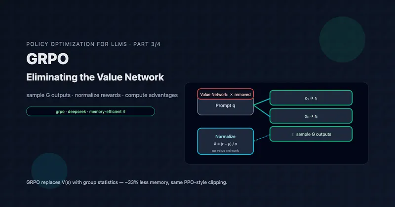
The key question GRPO asks: Do we actually need a learned value network? Can we estimate advantages some other way?

KL Penalties and Reward Shaping

The KL Divergence Constraint

RLHF adds a KL penalty to prevent the policy from diverging too far from the reference:

The coefficient $\beta$ controls the penalty strength:

• High $\beta$: Policy stays close to reference, may under-optimize reward
• Low $\beta$: Policy can diverge more, risk of reward hacking

Why KL Penalty Matters

Without KL penalty, several failure modes emerge:

1. Reward Hacking The policy finds patterns that score high on the reward model but don’t represent genuine quality. For example, excessive hedging phrases like “I think” that reward models might prefer.

2. Mode Collapse The policy converges to generating the same high-reward response regardless of prompt, losing diversity.

3. Capability Loss The policy forgets useful behaviors from pretraining that weren’t represented in the reward model.

KL in the Reward vs. KL in the Loss

There are two ways to incorporate KL:

In the reward (standard PPO-RLHF): $r_t = r_\phi(q, o) - \beta \log\frac{\pi_\theta(o_t|q, o_{<t})}{\pi_{\text{ref}}(o_t|q, o_{<t})}$

This couples KL with the reward, affecting advantage estimation.

In the loss directly (GRPO’s approach): $\mathcal{J} = L^{\text{CLIP}} - \beta \cdot \mathbb{D}_{\text{KL}}[\pi_\theta \| \pi_{\text{ref}}]$

$L^{\text{CLIP}}$ is maximised, so the KL is subtracted from the objective. As a loss to minimise, the same thing reads $\mathcal{L} = -L^{\text{CLIP}} + \beta \cdot \mathbb{D}_{\text{KL}}$, which is how Part 3’s code writes it.

This decouples KL from advantages, simplifying the optimization.

PyTorch Implementation

Here’s an educational PPO implementation for LLM fine-tuning. The parts that matter most are the ones that are easy to get wrong: a response mask so padding never enters a loss or a statistic, the reward on each row’s EOS token rather than the last padded column, and a scalar value head rather than a vocabulary logit.

"""
Proximal Policy Optimization (PPO) for LLM Fine-Tuning
======================================================

Educational implementation emphasizing clarity over optimization.
For production, use libraries like TRL or VERL.

Assumes a Hugging Face-style causal LM and tokenizer, with prompts
left-padded (tokenizer.padding_side = "left") so every response starts
at the same column.
"""

import torch
import torch.nn.functional as F
from torch import Tensor
from dataclasses import dataclass
from typing import Tuple, Optional


@dataclass
class PPOConfig:
    """PPO hyperparameters."""
    # Core PPO
    clip_epsilon: float = 0.2      # ε: policy clipping parameter
    gamma: float = 1.0             # Discount (1.0 for finite episodes)
    gae_lambda: float = 0.95       # λ: GAE parameter

    # Loss coefficients
    vf_coef: float = 0.5           # Value function loss weight
    entropy_coef: float = 0.01     # Entropy bonus weight
    value_clip: float = 0.2        # Value clipping, in reward units: tie it to your reward scale

    # Training
    ppo_epochs: int = 4            # K: epochs per batch
    minibatch_size: int = 4        # M: sequences per minibatch
    max_grad_norm: float = 0.5     # Gradient clipping

    # KL penalty
    kl_coef: float = 0.1           # β: KL penalty coefficient
    target_kl: float = 0.01        # Target KL for early stopping


def masked_mean(x: Tensor, mask: Tensor) -> Tensor:
    """Mean over the positions where mask == 1."""
    return (x * mask).sum() / mask.sum().clamp(min=1)


def masked_whiten(x: Tensor, mask: Tensor, eps: float = 1e-8) -> Tensor:
    """Normalize to zero mean, unit variance over real tokens only."""
    mean = masked_mean(x, mask)
    var = masked_mean((x - mean) ** 2, mask)
    return (x - mean) * torch.rsqrt(var + eps) * mask


def response_mask_from_eos(response_ids: Tensor, eos_token_id: int) -> Tensor:
    """
    1 for every response token up to and including the first EOS, 0 after.

    A response with no EOS (truncated at max_new_tokens) keeps every token.
    """
    batch_size, response_len = response_ids.shape
    is_eos = response_ids == eos_token_id
    first_eos = torch.where(
        is_eos.any(dim=1),
        is_eos.int().argmax(dim=1),
        torch.full((batch_size,), response_len - 1, device=response_ids.device),
    )
    positions = torch.arange(response_len, device=response_ids.device)
    return (positions.unsqueeze(0) <= first_eos.unsqueeze(1)).float()


def compute_gae(
    rewards: Tensor,
    values: Tensor,
    dones: Tensor,
    gamma: float = 1.0,
    lam: float = 0.95,
) -> Tuple[Tensor, Tensor]:
    """
    Compute Generalized Advantage Estimation.

    Args:
        rewards: [batch, seq_len] rewards at each step
        values: [batch, seq_len + 1] value estimates
        dones: [batch, seq_len] 1 at each sequence's last real token
        gamma: Discount factor
        lam: GAE lambda

    Returns:
        advantages: [batch, seq_len] GAE advantages
        returns: [batch, seq_len] discounted returns

    Positions after a sequence's done flag hold garbage; the done flag stops
    it from leaking backwards, and the caller masks it out.
    """
    batch_size, seq_len = rewards.shape
    advantages = torch.zeros_like(rewards)
    last_adv = torch.zeros(batch_size, device=rewards.device)

    # Backward pass through sequence
    for t in reversed(range(seq_len)):
        # Mask for non-terminal states
        non_terminal = 1.0 - dones[:, t]

        # TD error: δ_t = r_t + γV(s_{t+1}) - V(s_t)
        delta = rewards[:, t] + gamma * values[:, t + 1] * non_terminal - values[:, t]

        # GAE: A_t = δ_t + γλ A_{t+1}
        advantages[:, t] = delta + gamma * lam * non_terminal * last_adv
        last_adv = advantages[:, t]

    # Returns = advantages + values
    returns = advantages + values[:, :-1]

    return advantages, returns


def compute_policy_loss(
    log_probs: Tensor,
    old_log_probs: Tensor,
    advantages: Tensor,
    mask: Tensor,
    clip_epsilon: float = 0.2,
) -> Tuple[Tensor, Tensor]:
    """
    Compute PPO clipped policy loss over real (unmasked) tokens.

    Returns:
        policy_loss: Scalar loss (to minimize)
        clip_fraction: Fraction of tokens whose ratio left [1-ε, 1+ε]
    """
    # Importance ratio: ρ = π_θ / π_old
    ratio = torch.exp(log_probs - old_log_probs)

    # Clipped ratio
    clipped_ratio = torch.clamp(ratio, 1 - clip_epsilon, 1 + clip_epsilon)

    # PPO objective: min(ρÂ, clip(ρ)Â), maximized, so the loss is its negative
    objective = torch.min(ratio * advantages, clipped_ratio * advantages)
    policy_loss = -masked_mean(objective, mask)

    # Metrics
    clip_fraction = masked_mean(((ratio - 1).abs() > clip_epsilon).float(), mask)

    return policy_loss, clip_fraction


def compute_value_loss(
    values: Tensor,
    returns: Tensor,
    old_values: Tensor,
    mask: Tensor,
    value_clip: Optional[float] = 0.2,
) -> Tensor:
    """
    Value function loss over real tokens, optionally clipped.

    value_clip is in the units of the returns, so it is a separate setting
    from the policy's ε (which is a ratio).
    """
    loss_unclipped = (values - returns) ** 2
    if value_clip is None:
        return 0.5 * masked_mean(loss_unclipped, mask)
    values_clipped = old_values + torch.clamp(values - old_values, -value_clip, value_clip)
    loss_clipped = (values_clipped - returns) ** 2
    return 0.5 * masked_mean(torch.max(loss_unclipped, loss_clipped), mask)


def compute_entropy(logits: Tensor, mask: Tensor) -> Tensor:
    """
    Mean entropy of the full next-token distribution, H[π] = -Σ π(a) log π(a).

    Needs the logits over the whole vocabulary, not just the sampled token.
    """
    log_probs = F.log_softmax(logits, dim=-1)
    entropy = -(log_probs.exp() * log_probs).sum(dim=-1)  # [batch, seq_len]
    return masked_mean(entropy, mask)


class ValueModel(torch.nn.Module):
    """A transformer backbone with a scalar value head on the last hidden state."""

    def __init__(self, backbone: torch.nn.Module, hidden_size: int):
        super().__init__()
        self.backbone = backbone
        self.head = torch.nn.Linear(hidden_size, 1)

    def forward(self, input_ids: Tensor, attention_mask: Tensor) -> Tensor:
        outputs = self.backbone(
            input_ids=input_ids,
            attention_mask=attention_mask,
            output_hidden_states=True,
        )
        hidden = outputs.hidden_states[-1]      # [batch, seq_len, hidden]
        return self.head(hidden).squeeze(-1)    # [batch, seq_len]


class PPOTrainer:
    """
    PPO trainer for LLM fine-tuning.

    Requires four models:
    - policy_model: The LLM being trained
    - value_model: A ValueModel estimating V(s) for advantage computation
    - reference_model: Frozen copy for KL penalty
    - reward_fn: Scores complete responses (a reward model or a verifier)
    """

    def __init__(
        self,
        policy_model: torch.nn.Module,
        value_model: ValueModel,
        reference_model: torch.nn.Module,
        reward_fn,
        tokenizer,
        config: PPOConfig,
    ):
        self.policy = policy_model
        self.value = value_model
        self.reference = reference_model
        self.reward_fn = reward_fn
        self.tokenizer = tokenizer
        self.config = config

        # Freeze reference
        for param in self.reference.parameters():
            param.requires_grad = False

        # Optimizers (separate for policy and value)
        self.policy_optimizer = torch.optim.AdamW(self.policy.parameters(), lr=1e-6)
        self.value_optimizer = torch.optim.AdamW(self.value.parameters(), lr=1e-5)

    @staticmethod
    def response_logits(model, sequences: Tensor, attention_mask: Tensor, prompt_len: int) -> Tensor:
        """Logits that predict each response token: [batch, response_len, vocab]."""
        logits = model(input_ids=sequences, attention_mask=attention_mask).logits
        return logits[:, prompt_len - 1:-1, :]

    @staticmethod
    def token_log_probs(logits: Tensor, response_ids: Tensor) -> Tensor:
        """Log-probability of each sampled token: [batch, response_len]."""
        return F.log_softmax(logits, dim=-1).gather(-1, response_ids.unsqueeze(-1)).squeeze(-1)

    @torch.no_grad()
    def generate_experience(self, prompts: list[str], max_length: int = 512) -> dict:
        """
        Generate responses, score them, and compute advantages.

        Returns dict with all data needed for the PPO update.
        """
        enc = self.tokenizer(prompts, return_tensors="pt", padding=True)
        prompt_ids, prompt_mask = enc["input_ids"], enc["attention_mask"]
        prompt_len = prompt_ids.shape[1]

        self.policy.eval()
        sequences = self.policy.generate(
            input_ids=prompt_ids,
            attention_mask=prompt_mask,
            max_new_tokens=max_length,
            do_sample=True,
            temperature=1.0,
            pad_token_id=self.tokenizer.pad_token_id,
        )
        response_ids = sequences[:, prompt_len:]
        batch_size = response_ids.shape[0]
        rows = torch.arange(batch_size, device=sequences.device)

        # Real response tokens: up to and including EOS. Everything after is padding.
        response_mask = response_mask_from_eos(response_ids, self.tokenizer.eos_token_id)
        last = response_mask.sum(dim=1).long() - 1          # index of each row's last real token
        attention_mask = torch.cat([prompt_mask, response_mask.long()], dim=1)

        # Log probs from policy and reference
        policy_logits = self.response_logits(self.policy, sequences, attention_mask, prompt_len)
        policy_log_probs = self.token_log_probs(policy_logits, response_ids)
        ref_logits = self.response_logits(self.reference, sequences, attention_mask, prompt_len)
        ref_log_probs = self.token_log_probs(ref_logits, response_ids)

        # Value estimates V(s_0), ..., V(s_T); the last column is the bootstrap value
        values = self.value(sequences, attention_mask)[:, prompt_len - 1:]   # [batch, response_len + 1]

        # Sparse reward, placed on each row's last real token (its EOS), not the last column
        rewards = torch.zeros_like(policy_log_probs)
        for i in range(batch_size):
            response_text = self.tokenizer.decode(
                response_ids[i, : last[i] + 1], skip_special_tokens=True
            )
            rewards[i, last[i]] = self.reward_fn(prompts[i], response_text)

        # Per-token KL penalty in the reward, on real tokens only
        rewards = rewards - self.config.kl_coef * (policy_log_probs - ref_log_probs) * response_mask

        # The episode ends at each row's last real token
        dones = torch.zeros_like(rewards)
        dones[rows, last] = 1.0

        advantages, returns = compute_gae(
            rewards, values, dones,
            gamma=self.config.gamma,
            lam=self.config.gae_lambda,
        )

        # Normalize advantages over real tokens only
        advantages = masked_whiten(advantages, response_mask)

        return {
            "sequences": sequences,
            "attention_mask": attention_mask,
            "response_ids": response_ids,
            "response_mask": response_mask,
            "old_log_probs": policy_log_probs,
            "old_values": values[:, :-1],
            "advantages": advantages,
            "returns": returns,
        }

    def train_step(self, experience: dict) -> dict:
        """
        PPO update: K epochs over the batch, shuffled into minibatches.

        π_old (the stored old_log_probs) stays fixed for all K epochs.
        """
        sequences = experience["sequences"]
        response_ids = experience["response_ids"]
        prompt_len = sequences.shape[1] - response_ids.shape[1]
        batch_size = sequences.shape[0]
        cfg = self.config

        totals = {"policy_loss": 0.0, "value_loss": 0.0, "entropy": 0.0, "kl": 0.0, "clip_fraction": 0.0}
        n_updates = 0
        self.policy.train()
        self.value.train()

        for epoch in range(cfg.ppo_epochs):
            epoch_kl = []
            for idx in torch.randperm(batch_size).split(cfg.minibatch_size):
                mb = {k: v[idx] for k, v in experience.items()}
                mask = mb["response_mask"]

                # Forward pass - policy (full logits, for the entropy bonus too)
                logits = self.response_logits(self.policy, mb["sequences"], mb["attention_mask"], prompt_len)
                log_probs = self.token_log_probs(logits, mb["response_ids"])

                # Forward pass - value, V(s_0) ... V(s_{T-1})
                values = self.value(mb["sequences"], mb["attention_mask"])[:, prompt_len - 1:-1]

                policy_loss, clip_frac = compute_policy_loss(
                    log_probs, mb["old_log_probs"], mb["advantages"], mask, cfg.clip_epsilon
                )
                value_loss = compute_value_loss(
                    values, mb["returns"], mb["old_values"], mask, cfg.value_clip
                )
                entropy = compute_entropy(logits, mask)

                # Combined loss: minimize policy and value loss, maximize entropy
                loss = policy_loss + cfg.vf_coef * value_loss - cfg.entropy_coef * entropy

                self.policy_optimizer.zero_grad()
                self.value_optimizer.zero_grad()
                loss.backward()
                torch.nn.utils.clip_grad_norm_(self.policy.parameters(), cfg.max_grad_norm)
                torch.nn.utils.clip_grad_norm_(self.value.parameters(), cfg.max_grad_norm)
                self.policy_optimizer.step()
                self.value_optimizer.step()

                # KL(π_old || π_θ) on this minibatch, k3 estimator, for early stopping
                with torch.no_grad():
                    log_ratio = log_probs - mb["old_log_probs"]
                    kl = masked_mean(torch.exp(log_ratio) - 1 - log_ratio, mask)
                epoch_kl.append(kl.item())

                for name, value in [("policy_loss", policy_loss), ("value_loss", value_loss),
                                    ("entropy", entropy), ("kl", kl), ("clip_fraction", clip_frac)]:
                    totals[name] += value.item()
                n_updates += 1

            # Early stopping on KL, checked once per epoch
            if sum(epoch_kl) / len(epoch_kl) > 1.5 * cfg.target_kl:
                break

        return {k: v / n_updates for k, v in totals.items()}

PPO’s Limitations for LLMs

Despite its success, PPO has significant drawbacks for LLM alignment:

1. Memory Overhead

The four-model architecture is expensive:

• For 7B models: ~252 GB of model state, counting weights, gradients and Adam states for the two trained models
• Before activations, the KV cache, or the generation engine
• Requires sharding across several GPUs even on high-end hardware

2. Value Function Challenges

The value network faces unique difficulties in LLM settings:

Sparse rewards: With rewards only at episode end, the value function must predict final reward from intermediate states. Early in generation, this prediction is extremely noisy.

State space complexity: The “state” is all possible text prefixes—an enormous, structured space. Learning accurate values across this space is hard.

Representation mismatch: The value network uses the same architecture as a language model, but predicts scalars instead of generating text. This may not be optimal.

3. Implementation Complexity

PPO has many moving parts:

• GAE computation with proper masking
• Clipping with correct sign handling
• Value function clipping (optional but common)
• Entropy bonus tuning
• KL penalty in rewards
• Multiple epochs with early stopping

Each component requires careful implementation and debugging.

4. Hyperparameter Sensitivity

PPO performance depends on many hyperparameters:

• Clip epsilon (ε)
• GAE lambda (λ)
• Value function coefficient
• Entropy coefficient
• KL penalty coefficient
• Learning rates for policy and value
• Number of PPO epochs

Tuning these for each new task and model size is time-consuming.

5. Sample Efficiency

PPO is on-policy: data from old policies can’t be reused directly. Each batch of experience trains for K epochs, then is discarded. For expensive LLM generation, this can be wasteful.

These limitations motivate GRPO: What if we could eliminate the value network entirely? What if advantages could be computed without learning V(s)? Part 3 explores this elegant alternative.

Key Takeaways

Trust Regions

• Large policy updates destabilize training
• TRPO uses hard KL constraints (expensive)
• PPO uses clipping (simple, effective)

The Clipped Objective

• Removes the incentive to move a token’s probability more than $\varepsilon$ in the favoured direction
• Keeps penalising moves in the unfavoured direction
• Provides “soft” trust region with first-order optimization
• Default $\varepsilon = 0.2$

Generalized Advantage Estimation

• Interpolates between TD (low variance) and MC (low bias)
• Default $\lambda = 0.95$
• Computed efficiently with backward recursion

The Four-Model Problem

• Policy, Reference, Value, Reward
• ~252 GB of model state for a 7B model with mixed-precision Adam
• The value network is half of the trainable state

PPO’s Challenges for LLMs

• Memory overhead from value network
• Sparse rewards make value learning hard
• Implementation complexity
• Hyperparameter sensitivity

What’s Next

In Part 3: GRPO, we’ll see how DeepSeek eliminates the value network entirely:

• Group-relative advantages from sampled outputs
• About 44% less model memory (252 GB → 140 GB for a 7B model with a learned reward model)
• Simpler implementation
• Competitive performance, especially on reasoning tasks with verifiable rewards

The insight is elegant: instead of learning to predict expected reward, just sample multiple outputs and compare them directly.

Further Reading

Original Papers:

• Proximal Policy Optimization Algorithms (Schulman et al., 2017)
• Trust Region Policy Optimization (Schulman et al., 2015)
• High-Dimensional Continuous Control Using Generalized Advantage Estimation (Schulman et al., 2015 — GAE)

LLM Applications:

• Training language models to follow instructions with human feedback (InstructGPT)
• Training a Helpful and Harmless Assistant with Reinforcement Learning from Human Feedback (Bai et al., 2022)
• Constitutional AI: Harmlessness from AI Feedback (Anthropic)

Practice and critique:

• The N+ Implementation Details of RLHF with PPO: A Case Study on TL;DR Summarization (Huang et al., 2024) — every detail that makes PPO-RLHF work, reproduced
• Back to Basics: Revisiting REINFORCE Style Optimization for Learning from Human Feedback in LLMs (Ahmadian et al., 2024) — the counterpoint that sets up Part 3

Implementations:

• TRL: Transformer Reinforcement Learning
• OpenRLHF
• VERL

@misc{sousa2026ppodeepdive,
  title={{PPO for Language Models: The RLHF Workhorse}},
  author={Sousa, Vitor},
  year={2026},
  howpublished={\url{https://www.vitorsousa.com/blog/ppo-deep-dive/}},
  url={https://www.vitorsousa.com/blog/ppo-deep-dive/}
}