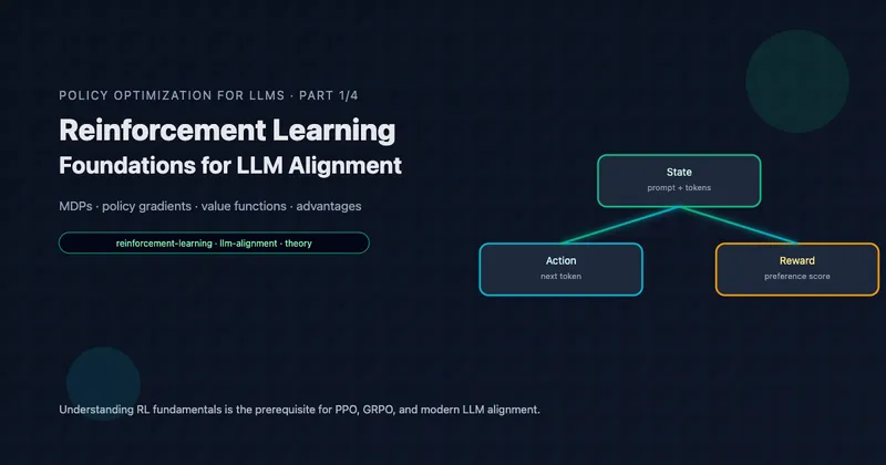
Reinforcement Learning Foundations for LLM Alignment

Part 1 of 4: The Mathematical Foundations

TL;DR: Before understanding PPO, GRPO, or any modern LLM alignment algorithm, you need solid RL foundations. This article covers MDPs, policy gradients, the variance problem, value functions, Bellman equations, and advantage estimation—all through the lens of language model fine-tuning. By the end, you’ll understand why these algorithms are designed the way they are.

Reading time: ~35 minutes

Why RL for Language Models?

You’ve trained a language model on terabytes of text. It can complete sentences, answer questions, even write code. But it also happily generates harmful content, confidently states falsehoods, and ignores user preferences. Supervised fine-tuning on curated examples helps, but you can’t enumerate every possible good response.

What you need is a way to optimize for “goodness” directly—to tell the model “responses like this are better than responses like that” and have it learn the pattern. This is exactly what reinforcement learning provides.

The insight behind RLHF (Reinforcement Learning from Human Feedback) is powerful: instead of showing the model correct outputs, we show it a reward signal indicating how good its outputs are. The model then learns to maximize this reward.

But RL for LLMs isn’t straightforward. The action space is enormous (vocabulary size per token), episodes are variable length, rewards are sparse (often only at generation end), and we need stable training for billion-parameter models.

Understanding the foundations deeply will help you see why algorithms like PPO and GRPO make specific design choices—and when those choices might not be right for your problem.

Table of Contents

1. The MDP Framework
2. Policies and the Objective
3. Policy Gradients: Learning Without a Model
4. The Variance Problem
5. Value Functions and Bellman Equations
6. Advantage Functions: The Key Insight
7. Actor-Critic Methods
8. From General RL to LLM Fine-Tuning
9. Key Takeaways

The MDP Framework

Reinforcement learning formalizes sequential decision-making through Markov Decision Processes (MDPs). Understanding this framework precisely will help you see how LLM generation maps onto RL concepts.

Definition

An MDP is defined by the tuple $(\mathcal{S}, \mathcal{A}, P, R, \gamma)$:

The Markov Property

The “Markov” in MDP refers to the Markov property: the future depends only on the current state, not on how we got there.

$P(s_{t+1} | s_t, a_t, s_{t-1}, a_{t-1}, \ldots) = P(s_{t+1} | s_t, a_t)$

This is crucial for tractability—we don’t need to remember the entire history, just the current state.

The Agent-Environment Loop

At each timestep $t$:

1. Agent observes state $s_t$
2. Agent selects action $a_t$ according to its policy
3. Environment transitions to $s_{t+1} \sim P(\cdot | s_t, a_t)$
4. Agent receives reward $r_t = R(s_t, a_t, s_{t+1})$
5. Repeat until terminal state or horizon

LLM Generation as an MDP

For language model fine-tuning, we can map concepts as follows:

The state space is enormous (all possible token sequences up to context length), and the action space is the vocabulary size (typically 32K-128K tokens). This scale motivates many of the algorithmic choices we’ll see.

Key Insight: The Markov property technically holds for LLM generation—the next token distribution depends only on the current sequence, not on how we generated it. However, the state itself encodes the full history, so we’re not actually discarding information.

Policies and the Objective

What is a Policy?

A policy $\pi$ maps states to actions. It can be:

• Deterministic: $a = \pi(s)$ — always the same action in state $s$
• Stochastic: $a \sim \pi(a|s)$ — a probability distribution over actions

For LLMs, the policy is inherently stochastic: $\pi_\theta(o_t | s_t) = \pi_\theta(o_t | q, o_{<t})$ is the probability of token $o_t$ given the context. The parameters $\theta$ are the model weights.

The Return

The return $G_t$ is the cumulative (discounted) reward from time $t$ onwards:

$G_t = \sum_{k=0}^{\infty} \gamma^k r_{t+k} = r_t + \gamma r_{t+1} + \gamma^2 r_{t+2} + \cdots$

The discount factor $\gamma$ serves multiple purposes:

• Mathematical: Ensures the sum converges for infinite horizons
• Practical: Encodes preference for immediate vs. delayed rewards
• LLM setting: Often $\gamma = 1$ since episodes are finite

The RL Objective

The goal of RL is to find a policy that maximizes expected return:

$J(\theta) = \mathbb{E}_{\tau \sim \pi_\theta}\left[\sum_{t=0}^{T} \gamma^t r_t\right] = \mathbb{E}_{\tau \sim \pi_\theta}[G_0]$

where $\tau = (s_0, a_0, r_0, s_1, a_1, r_1, \ldots)$ is a trajectory sampled by following policy $\pi_\theta$.

The expectation is over:

• Initial state distribution $s_0 \sim \rho_0$
• Actions from policy $a_t \sim \pi_\theta(a|s_t)$
• Transitions from dynamics $s_{t+1} \sim P(s'|s_t, a_t)$

For LLMs Specifically

In the LLM setting, the objective simplifies to:

$J(\theta) = \mathbb{E}_{q \sim P(Q), \, o \sim \pi_\theta(O|q)}[R(q, o)]$

where:

• $q$ is a prompt from the prompt distribution $P(Q)$
• $o = (o_1, \ldots, o_T)$ is a complete response sampled from the model
• $R(q, o)$ is the reward (typically from a reward model)

With sparse rewards (only at episode end), there’s no discounting to worry about within an episode.

Policy Gradients: Learning Without a Model

How do we optimize $J(\theta)$? We can’t compute it analytically—it requires integrating over all possible trajectories. But we can estimate its gradient and use gradient ascent.

The Policy Gradient Theorem

The policy gradient theorem (Sutton et al., 1999) provides a remarkable result: we can estimate $\nabla_\theta J(\theta)$ using only samples, without knowing the transition dynamics $P$.

$\nabla_\theta J(\theta) = \mathbb{E}_{\tau \sim \pi_\theta}\left[\sum_{t=0}^{T} \nabla_\theta \log \pi_\theta(a_t|s_t) \cdot G_t\right]$

Let’s unpack this:

• $\nabla_\theta \log \pi_\theta(a_t|s_t)$ is the score function—the direction that increases the probability of action $a_t$
• $G_t$ is the return from time $t$—how good the outcome was
• The product says: “increase probability of actions that led to high returns”

Intuition: Credit Assignment

The gradient has an elegant interpretation:

1. Sample a trajectory by running the policy
2. For each action taken, compute how much total reward followed
3. If reward was high, increase that action’s probability
4. If reward was low, decrease that action’s probability

This is the core of policy gradient methods: reinforce good actions, discourage bad ones.

The REINFORCE Algorithm

The simplest policy gradient algorithm is REINFORCE (Williams, 1992):

Algorithm: REINFORCE

For each episode:
    1. Sample trajectory τ = (s₀, a₀, r₀, ..., s_T, a_T, r_T) using π_θ
    
    2. For t = 0 to T:
        Compute return: G_t = Σₖ γᵏ r_{t+k}
    
    3. Compute gradient estimate:
        ∇̂ = Σₜ ∇_θ log π_θ(aₜ|sₜ) · Gₜ
    
    4. Update: θ ← θ + α∇̂

Why This Works: The Log-Derivative Trick

The derivation uses the log-derivative trick:

$\nabla_\theta \pi_\theta(a|s) = \pi_\theta(a|s) \cdot \nabla_\theta \log \pi_\theta(a|s)$

This converts a gradient of a probability into an expectation we can sample:

$\nabla_\theta \mathbb{E}_{a \sim \pi_\theta}[f(a)] = \mathbb{E}_{a \sim \pi_\theta}[f(a) \cdot \nabla_\theta \log \pi_\theta(a|s)]$

The full derivation for trajectories is more involved but follows the same principle.

Key Insight: Policy gradients are model-free—we don’t need to know $P(s'|s,a)$. We only need to sample from the environment and observe rewards. This is crucial for LLMs where the “environment” is just string concatenation.

The Variance Problem

REINFORCE is elegant but has a critical flaw: high variance. The gradient estimates are so noisy that learning is impractically slow.

Sources of Variance

Consider what affects the gradient estimate $\nabla_\theta \log \pi_\theta(a_t|s_t) \cdot G_t$:

1. Stochastic policy: Different action samples give different gradients
2. Stochastic transitions: Same action can lead to different states
3. Long horizons: $G_t$ includes all future rewards, accumulating randomness
4. Sparse rewards: Most of the signal comes from rare events

A Concrete Example

Suppose you’re training an LLM to solve math problems. The reward is +1 for correct, 0 for incorrect.

Episode 1: Model generates a correct solution. Every token gets gradient proportional to +1.

Episode 2: Model generates an incorrect solution. Every token gets gradient proportional to 0.

The problem: In episode 1, all tokens get positive reinforcement—including lucky guesses, unnecessary steps, and tokens that happened to work but weren’t essential. The gradient doesn’t distinguish “this token was crucial” from “this token was irrelevant.”

Variance Reduction with Baselines

A key insight: we can subtract any baseline $b(s_t)$ that doesn’t depend on actions without changing the expected gradient:

$\nabla_\theta J(\theta) = \mathbb{E}\left[\sum_{t} \nabla_\theta \log \pi_\theta(a_t|s_t) \cdot (G_t - b(s_t))\right]$

Why doesn’t this change the expectation?

$\mathbb{E}_{a \sim \pi}\left[\nabla_\theta \log \pi_\theta(a|s) \cdot b(s)\right] = b(s) \cdot \mathbb{E}_{a \sim \pi}\left[\nabla_\theta \log \pi_\theta(a|s)\right] = b(s) \cdot \nabla_\theta \sum_a \pi_\theta(a|s) = b(s) \cdot \nabla_\theta 1 = 0$

The baseline can be anything that doesn’t depend on the action—but choosing it well dramatically reduces variance.

Optimal Baseline

The variance-minimizing baseline is approximately the expected return from state $s_t$:

$b^*(s_t) \approx \mathbb{E}[G_t | s_t]$

This is the value function $V(s_t)$, which we’ll explore next.

Intuition: Relative Performance

With a good baseline, the gradient update becomes:

$\nabla_\theta \log \pi_\theta(a_t|s_t) \cdot (G_t - V(s_t))$

This says:

• If $G_t > V(s_t)$: Action was better than expected → increase probability
• If $G_t < V(s_t)$: Action was worse than expected → decrease probability
• If $G_t = V(s_t)$: Action was exactly as expected → no change

This relative signal is far more informative than absolute returns.

Key Insight: The baseline transforms absolute returns into relative performance measures. This is the foundation of advantage-based methods—and explains why GRPO’s group normalization works.

Value Functions and Bellman Equations

To use $V(s)$ as a baseline, we need to estimate it. Value functions are central to RL and worth understanding deeply.

State Value Function

The state value function $V^\pi(s)$ is the expected return starting from state $s$ and following policy $\pi$:

$V^\pi(s) = \mathbb{E}_\pi\left[\sum_{k=0}^{\infty} \gamma^k r_{t+k} \,\Big|\, s_t = s\right]$

This answers: “How good is it to be in state $s$?”

Action Value Function

The action value function (or Q-function) $Q^\pi(s, a)$ is the expected return starting from state $s$, taking action $a$, then following policy $\pi$:

$Q^\pi(s, a) = \mathbb{E}_\pi\left[\sum_{k=0}^{\infty} \gamma^k r_{t+k} \,\Big|\, s_t = s, a_t = a\right]$

This answers: “How good is it to take action $a$ in state $s$?”

Relationship Between V and Q

The value function is the expected Q-value under the policy:

$V^\pi(s) = \mathbb{E}_{a \sim \pi}[Q^\pi(s, a)] = \sum_a \pi(a|s) Q^\pi(s, a)$

The Bellman Equation

Value functions satisfy a recursive relationship called the Bellman equation:

$V^\pi(s) = \mathbb{E}_{a \sim \pi, s' \sim P}\left[r(s, a, s') + \gamma V^\pi(s')\right]$

This says: “The value of a state equals the expected immediate reward plus the discounted value of the next state.”

For Q-functions:

$Q^\pi(s, a) = \mathbb{E}_{s' \sim P}\left[r(s, a, s') + \gamma \sum_{a'} \pi(a'|s') Q^\pi(s', a')\right]$

Why Bellman Equations Matter

The Bellman equation enables bootstrapping: we can estimate $V(s)$ using our current estimate of $V(s')$, without waiting for the episode to end.

Monte Carlo: Wait for episode end, compute $G_t = \sum_k \gamma^k r_{t+k}$, update $V(s_t) \leftarrow V(s_t) + \alpha(G_t - V(s_t))$

Temporal Difference (TD): After one step, update using $V(s_t) \leftarrow V(s_t) + \alpha(r_t + \gamma V(s_{t+1}) - V(s_t))$

TD learning has lower variance (one-step update vs. full episode) but introduces bias (using an estimate $V(s_{t+1})$ instead of the true expected return).

TD Error

The TD error is the difference between our estimate and the bootstrapped target:

$\delta_t = r_t + \gamma V(s_{t+1}) - V(s_t)$

If our value function is accurate, $\mathbb{E}[\delta_t] = 0$. The TD error measures how “surprised” we are by what happened.

Key Insight: Bellman equations let us learn value functions incrementally, updating after each step rather than waiting for episodes to complete. This is especially valuable for long episodes like LLM generation.

Advantage Functions: The Key Insight

The advantage function combines V and Q to measure how much better an action is than average:

$A^\pi(s, a) = Q^\pi(s, a) - V^\pi(s)$

Interpretation

• $A(s, a) > 0$: Action $a$ is better than the average action in state $s$
• $A(s, a) < 0$: Action $a$ is worse than average
• $A(s, a) = 0$: Action $a$ is exactly average

The advantage answers the crucial question: “Is this action better or worse than what I’d typically do?”

Why Advantages for Policy Gradients?

Using advantages in the policy gradient gives:

$\nabla_\theta J(\theta) = \mathbb{E}\left[\sum_t \nabla_\theta \log \pi_\theta(a_t|s_t) \cdot A^\pi(s_t, a_t)\right]$

This is optimal for variance reduction because:

1. $\mathbb{E}_a[A(s, a)] = 0$ by construction (advantages are centered)
2. The signal focuses on relative action quality
3. It separates “was the action good?” from “was the state good?”

Estimating Advantages

We rarely know $A^\pi$ exactly. Common estimators:

1. Monte Carlo Advantage: $\hat{A}_t = G_t - V(s_t)$ Use actual returns minus estimated value. Unbiased but high variance.

2. TD Advantage: $\hat{A}_t = r_t + \gamma V(s_{t+1}) - V(s_t) = \delta_t$ One-step TD error. Low variance but biased.

3. Generalized Advantage Estimation (GAE): $\hat{A}_t^{\text{GAE}(\gamma, \lambda)} = \sum_{k=0}^{\infty} (\gamma\lambda)^k \delta_{t+k}$ Interpolates between MC ($\lambda=1$) and TD ($\lambda=0$). We’ll explore GAE deeply in Part 2.

Properties of Good Advantage Estimators

There’s typically a bias-variance tradeoff: lower variance estimators introduce more bias (by relying on learned value functions).

Key Insight: The advantage function is the “right” quantity for policy gradients. It tells us exactly what we want to know: was this action better or worse than average? All modern policy optimization methods (PPO, GRPO, etc.) are fundamentally about estimating advantages well.

Actor-Critic Methods

Actor-critic methods combine policy gradients (the “actor”) with learned value functions (the “critic”). This architecture underlies PPO and most modern RL algorithms.

The Two Components

Actor: The policy $\pi_\theta(a|s)$ that selects actions

• Parametrized by $\theta$
• Optimized via policy gradients
• Goal: maximize expected return

Critic: The value function $V_\psi(s)$ or $Q_\psi(s, a)$

• Parametrized by $\psi$
• Optimized via Bellman equation (TD learning)
• Goal: accurately estimate expected returns

Why Two Networks?

Each component benefits the other:

1. Critic helps actor: Provides baseline/advantage estimates for lower-variance policy gradients
2. Actor helps critic: Generates on-policy data for value function training

The A2C Algorithm

Advantage Actor-Critic (A2C) is a foundational actor-critic algorithm:

Algorithm: A2C

For each batch of experience:
    1. Collect trajectories using current policy π_θ
    
    2. Compute advantages:
        For each timestep t:
            δ_t = r_t + γV_ψ(s_{t+1}) - V_ψ(s_t)  # TD error
            (Or use GAE for multi-step advantages)
    
    3. Update critic (minimize value loss):
        L_critic = Σ_t (V_ψ(s_t) - G_t)²  # Or TD targets
        ψ ← ψ - α_critic ∇_ψ L_critic
    
    4. Update actor (maximize policy objective):
        L_actor = Σ_t log π_θ(a_t|s_t) · Â_t
        θ ← θ + α_actor ∇_θ L_actor

On-Policy vs. Off-Policy

On-policy methods (A2C, PPO, GRPO) require data from the current policy:

• Samples from $\pi_\theta$ used to update $\pi_\theta$
• Must discard data after each update
• Simpler theory but less sample efficient

Off-policy methods (DQN, SAC) can reuse old data:

• Samples from any policy can update $\pi_\theta$
• Requires importance sampling or replay buffers
• More sample efficient but more complex

LLM fine-tuning typically uses on-policy methods because:

1. The state space (text) is too large for replay buffers
2. On-policy methods are more stable for large models
3. Sample efficiency matters less when each “sample” is a full text generation

Challenges in Actor-Critic

1. Training instability: Actor and critic must improve together; if one diverges, both fail
2. Sample efficiency: On-policy methods need fresh samples after each update
3. Hyperparameter sensitivity: Learning rates, advantage estimation, entropy bonuses all interact
4. Scale: For LLMs, the critic is another massive network to train

Key Insight: Actor-critic methods are powerful but complex. The critic provides essential variance reduction, but at the cost of doubled model capacity and potential instability. This motivates GRPO’s approach of eliminating the critic entirely.

From General RL to LLM Fine-Tuning

Let’s map everything we’ve learned to the specific setting of language model alignment.

The LLM-RL Correspondence

Unique Challenges for LLMs

1. Enormous Action Space

Vocabulary sizes of 32K-128K tokens mean:

• Can’t enumerate all actions
• Must use function approximation (the LLM itself)
• Exploration is implicit in stochastic sampling

2. Sparse Rewards

Typically, reward comes only at generation end:

• $r_t = 0$ for $t < T$
• $r_T = R(q, o)$ — the reward model score

This makes credit assignment hard: which tokens were responsible for the reward?

3. Variable-Length Episodes

Generations can be 10 tokens or 1000 tokens:

• Can’t use fixed-horizon methods
• Must handle EOS token properly
• Padding and masking complexities

4. The Reference Model Constraint

Unlike standard RL, we don’t want to maximize reward unconditionally. We want to improve while staying close to a reference model:

$\max_\theta \mathbb{E}[R(q, o)] - \beta \cdot \text{KL}(\pi_\theta || \pi_{\text{ref}})$

This prevents:

• Reward hacking: Finding exploits in the reward model
• Mode collapse: Generating the same high-reward response always
• Capability loss: Forgetting useful behaviors from pretraining

5. Scale

Training billion-parameter models requires:

• Massive memory for model weights, gradients, optimizer states
• Distributed training across many GPUs
• Careful numerical stability

The RLHF Pipeline

What’s Coming Next

With these foundations, we’re ready to understand PPO (Part 2):

• How clipping provides stable updates
• How GAE estimates advantages
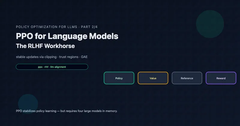
• Why it requires four models
• And why that’s a problem

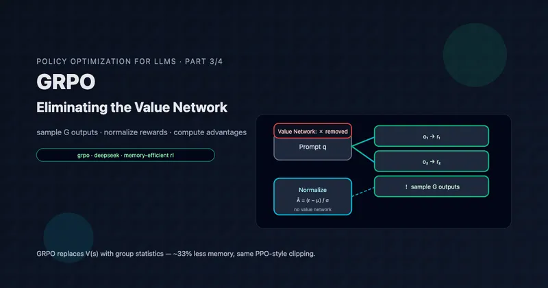
Then GRPO (Part 3) will show how to eliminate the critic by clever use of group statistics.

Finally, GDPO (Part 4) will address multi-reward settings where GRPO falls short.

Key Takeaways

The MDP Framework

• RL formalizes sequential decisions as states, actions, rewards
• Markov property: future depends only on current state
• LLM generation maps naturally to this framework

Policy Gradients

• We can optimize expected reward using gradient ascent
• The policy gradient theorem enables learning without knowing dynamics
• REINFORCE is simple but high-variance

The Variance Problem

• Raw policy gradients are too noisy for practical use
• Baselines reduce variance without changing expected gradient
• The optimal baseline is approximately the value function

Value Functions

• $V(s)$ = expected return from state $s$
• $Q(s,a)$ = expected return from state $s$ taking action $a$
• Bellman equations enable bootstrapped learning

Advantage Functions

• $A(s,a) = Q(s,a) - V(s)$ measures relative action quality
• Advantages are centered: $\mathbb{E}_a[A(s,a)] = 0$
• This is the key quantity for policy optimization

Actor-Critic

• Actor (policy) + Critic (value function) work together
• Critic provides variance reduction for actor updates
• Doubles the model capacity required

LLM-Specific Considerations

• Sparse rewards make credit assignment hard
• Reference model constraint prevents reward hacking
• Scale demands memory-efficient algorithms

What’s Next

In Part 2: PPO for Language Models, we’ll see how Proximal Policy Optimization addresses many challenges:

• Trust regions for stable updates
• GAE for flexible advantage estimation
• Clipping for simplicity

But we’ll also see PPO’s costs: the four-model architecture that strains GPU memory, and the complexity that makes implementation tricky. This sets the stage for GRPO’s elegant simplification.

Further Reading

Foundational Papers:

• Policy Gradient Methods for Reinforcement Learning with Function Approximation (Sutton et al., 1999)
• Simple Statistical Gradient-Following Algorithms for Connectionist Reinforcement Learning (Williams, 1992 — REINFORCE)

Textbooks:

• Reinforcement Learning: An Introduction (Sutton & Barto, 2018) — The definitive reference
• Deep Reinforcement Learning (Foundations and Trends survey)

LLM-Specific:

• Training language models to follow instructions with human feedback (InstructGPT, Ouyang et al., 2022)
• Learning to summarize from human feedback (Stiennon et al., 2020)